Optimising LimeSDR matching for HF

This post is in response to comments from some of our backers who are mainly interested in working with frequencies below 100MHz.

Firstly, we would like to highlight the fact that it is not possible to achieve optimum performance across the entire operating range of LimeSDR — all the way from 100kHz to 3.8GHz — with only a single matching network.

Second to which we would note that the 1.2 hardware version which was shipped to our beta testing community of around 100 people, has the exact same matching network as the version 1.4 hardware that is being shipped today. We decided to stick with the same network since the reviews of the 1.2 hardware were positive and lead to about 30 or so use cases for the board in all manner of applications.

Optimising matching

The default matching network on the LimeSDR RX1_L input is optimized for good return loss at around 900MHz, where the majority of applications reside. This means non-optimal performance in the HF band. In order to satisfy the need for a high level of sensitivity below 100MHz, there are a number of solutions that could be adopted on either RX1_L or the Broadband RX1_W and RX2_W ports, depending upon particular use and preferences.

Table A. Component Values for the LimeSDR RX1_L input.

Table A gives a number of examples on how the RX1_L input can be modified from the default component values for better performance at HF. The EasyFix1 solution gives substantial improvement in HF performance with the least amount of reworking. The EasyFix2 solution has a better noise figure, and uses easily obtainable components. The broadband solution provides good VSWR over broad range of frequencies with a small Noise Figure penalty (around 2.5dB).

The measured performance of the networks of Table A are shown in Figure 1 and Figure 2.

Figure 1 shows the digital output level of the receiver in dBFS, as the input frequency is swept from 100kHz to 1GHz with a constant input level of -45dBm. It can be seen that the default network has around 40dB less output in the HF band (3-30MHz). All networks show a fall in level below 30MHz due to internal design of the LMS7002M. The LNA gain is set to 0 (Maximum), and the PGA gain is set to 0dB. This was to ensure the receiver did not saturate around 800MHz. For HF operation, higher PGA gain would be possible.

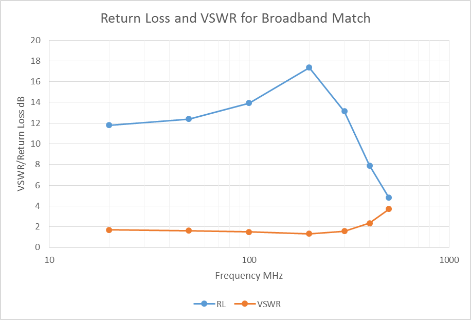
Figure 2 shows the Return Loss and VSWR of the Broadband network from 20MHz to 500MHz. The matching network forms a terminated differential transmission line, and has good performance from 30MHz to 400MHz. The lower frequency is set by the 100nF capacitor C14. Note 1pF and 82R resistor are in parallel and soldered on top of each other. The Noise figure of the same network was measured on an evaluation board and found to be 10dB at 30MHz and 6dB at 100MHz. It is possible to further optimize component values in circuit simulators such as NGSPICE and other simulators to trade noise figure, gain and return loss.

The broadband matching network can also be applied to the wideband ports of the LimeSDR. Table B shows some example component values that can be used on RX1_W and RX2_W. In Figure 3 we show results for the matching networks of Table B. Here, the LNA gain is set to 0 (Maximum), and the PGA gain is set to +19dB. The observed behaviour is very similar to that seen for RX1_L. Both networks give reasonable return loss below 400MHz.

Table B Component Values for the LimeSDR RX1_W and RX2_W inputs.

In a future post we will provide a guide to locating and replacing the simple passive components identified here.