Welcome to the ninth episode in the LimeSDR Made Simple series. Since the first we’ve been gradually adding more tools to the SDR toolbox and if you have followed the series along, by now the operation of the LimeSDR should be well and truly demystified.
Last time we looked at C code and how to make a simple frequency scanner. This time we will look at pyLMS7002M, a python library for the LimeSDR. Rather than try to make something this time we will look at a poorly understood example, the VNA!
Note that this is not going to be a calibrated, highly accurate VNA — like equipment from Rohde & Schwarz and costing more than a luxury car — but it does work to give an indication of how a circuit will look at a given frequency.
Some assembly required and for this example we will need the following items:
- A directional coupler
- SMA leads
- An SMA attenuator (preferably 10dB)
- An SMA “calibrated” short
Getting set up
The VNA example has a few dependencies, however the setup isn’t too complex. First make sure you have a valid and working LimeSDR installation (Linux or windows). At the time of writing you will also need Python 2.7.x and Python 3.x installs.
Next head to https://github.com/myriadrf/pyLMS7002M/ and for the purpose of this article we used this version, which must be installed for Python 2.7.x. There is also a Python 3.x branch, but this has not been fully tested yet and so using the master branch is recommended.
pySmithPlot can be found here: https://github.com/vMeijin/pySmithPlot and the version we used was this one. Git clone or download these files and place them in a suitable directory.
First we need to install pyLMS7002M. Navigate to the folder in a terminal (“cmd” in windows).
There should be a “setup.py” in the directory it can be installed by the command “python2 setup.py install”. Note the use of python2 to force the older version.
Next for pySmithPlot follow a similar procedure to install, only this time be sure to install this with “python3 setup.py install”. On a Windows install we did have to pull in some of the dependencies manually via “pip” and this may vary with different systems.
Install complete
At this point the VNA should work and allow the generation of s.2p files (S-Parameters), but will not show a smith plot which is kind of key for a VNA.
In the pyLMS7002M directory there are a few examples split into two directory’s basic and VNA, the first to try is in basic called “findLimeSDR.py” which essentially does as it says in the label. Run this example by the command “python2 findLimeSDR.py” and the output should look something like:

This will prove the pyLMS7002M library is working. So let’s move on to the VNA example.
The VNA works in two parts: measure and calculate. As you would expect the first thing we need to do is measure. But before we start we need to set-up the hardware. The docs come in handy here and provide a useful picture:

Going from left to right, we need to connect the TX to TX2_1 on the LimeSDR. The RX connects to RX1_H. There is a 10dB attenuator and this in theory can be another value as it is calibrated out. It is there to provide a fixed impedance and control output power, which will reduce the effects of load changes and improve the measurement accuracy.
The directional coupler
This is likely the hardest part of the setup to source. Without going too deep into transmission line theory a directional coupler does two things:
- Coupling
- Directionality
One path goes from in to out and that is the main signal path. This path is coupled to the third terminal via a variety of methods (e.g. strip-line and waveguide etc.) There is a nice guide to them here. This essentially results in a smaller version of the signal appearing on the coupled connection.
Directionality is achieved by terminating one of the coupled paths with a matched impedance. This will absorb most of the energy in that direction, meaning that only signals passing in one direction will be emitted from the coupled port.
This may have got you thinking, can we make a directional coupler and the answer is yes, but it will not be calibrated and the coupling and directionality not be guaranteed. Stripline versions can be as simple as two parallel tracks with an single ended impedance of 50R (for the LimeSDR, but there are 75R systems too). One of the outputs will be 50R to ground and the other is the coupled port.
As you can imagine there are a few key aspects with the directional coupler that matter: the amount of signal coupled, its directivity and finally the loss. The recommended coupler is a Mini Circuits ZHDC-16-63-S+. This has around 30dB directivity, which is the ratio of how much signal is isolated to passed, e.g. how much the directional coupler sees in either direction. The mainline loss is 2dB, which is the loss of signal from in to out. The coupling amount is 17dB.
We didn’t have a Mini Circuits coupler to-hand and so we used an AtlanTecRF A2023-20. This posed a few issues: firstly, iy is only a 500MHz to 2GHz coupler, and secondly it only has around 25 dB directivity.
This poses another problem as the example is by default configured to use 2.4GHz, so we needed to change this to something more suitable for our coupler and we chose 1.5GHz. It’s important to bear in mind that near the edges of the LNAH bandwidth there are a few issues, so it’s best to stay well within a band or change the impedance matching stage so that it’s well match for the frequency being measured. This can become a bit chicken and egg, as the VNA is the tool to help with this.
For example, we did have issues with phase noise on the LNAH input and when trying to get an accurate measurement at 866MHz this was near impossible.
If you just read this whole segment and it didn’t mean much you may want to revisit episode 2 of the LimeSDR Made Simple series as we discuss matching there.
First measurement
Before we start we need to adjust the frequency. Note that the default LNA chosen is the LNAH path, this should really be 1500MHz+ going below this will reduce sensitivity.
Opening “measureVNA.py” we need to alter the following lines (match these to your requirements):
startFreq = 2.3e9
endFreq = 2.4e9
nPoints = 101
to
startFreq = 1500e6
endFreq = 1510e6
nPoints = 101
Saving the file we can now run the example “python2 measureVNA.py test1”
This will give quite a lot of feedback in the command line, but will ask for a short to start with and this is the calibration step.

This first step will calibrate the VNA to the short applied. It’s best to use a “calibrated short” for this. One of the things that can be hard to imagine is that at RF frequency a short can be something quite other than a short. The stray inductance and capacitance in a wire or PCB can form whole circuits and if you don’t believe me go look at a WiFi antenna and do a ohmic test with a meter.
After this calibration step is completed the script will ask for the DUT (Device Under Test).

This will then run the same set of tests as the calibration. In very simplistic terms the VNA works by comparing the phase and magnitude of these two values to calculate the losses from reactance (imaginary) and resistance (real). This is then plotted in a special chart designed to show this information clearly, called a Smith Chart.
After this test is complete we should have two text files saved called:
vna_test1_short_1500000000.0_1510000000.0_101
vna_test1_DUT_1500000000.0_1510000000.0_101
Plotting the results
Next we need to process these files into a S-Parameter and a set of plots. This is where there are a few modifications to the code required.
In the “calculateVNA.py” example we need to change the following lines to allow the smithplot.py version 0.2.0 support.
Change the line:
from smithplot.smithaxes import update_scParams
to:
from smithplot.smithaxes import SmithAxes
Near the bottom of the file:
subplot(1, 1, 1, projection=’smith’,grid_major_fancy=True,
grid_minor_fancy=True, plot_hacklines=True)
to
subplot(1, 1, 1, projection=’smith’,grid_major_fancy=True,
grid_minor_fancy=True)
This should be a sufficient change to get the example working.
Next run the command “python3 calculateVNA.py test1 plot”

The first plot is the calibrated short phase. This should have small changes with frequency and if the DUT is a short it should be an identical match.

Just like the “short” phase plot, this shows phase vs. frequency. Phase changes are introduced when there is a reactive component to the load. Simply put the phase difference between the short and DUT will be compared and this gives the reactive part of the Smith Chart.

This is the Voltage Standing Wave Ratio, which is a measure of the transmitted power.

This is the S11 S-Parameter plot, which is the amount of power reflected from the load.

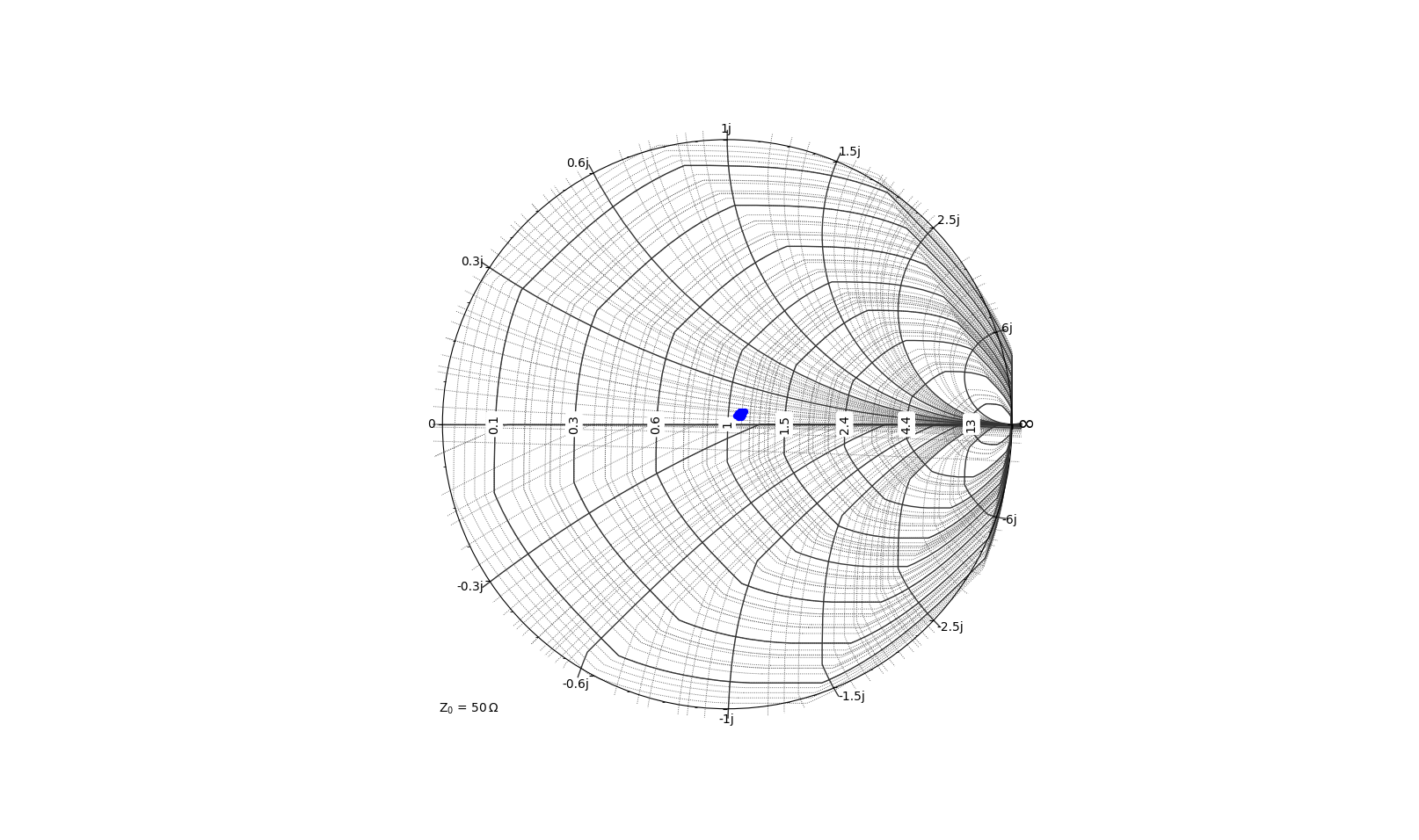
Last but not least is the Smith plot, which is a special chart that shows what the load looks like in terms of reactive and resistive components. There is a good introduction to Smith Chart basics here.
Final Words
Hopefully the LimeSDR Made Simple series of articles have been of use. At this point we’ve handed the keys to one of the most useful RF engineering tools available, the VNA.
From our experience this example could be improved with a little more RF power, and a good external LNA could be used. We also noticed that with larger attenuators we were getting some odd results with phase changes, likely due to the received signal sat in the noise floor.
All that is left to do is start to use some of the tips and tricks to start making incredible SDR applications, much like this VNA example!
Karl Woodward