This is the third in a series of posts that aims to make the LimeSDR platform a little more approachable. Again we will build upon previous examples and if you missed the last in the series it is available here.
Last time we looked at the RX stage in detail with the aim of understanding a good proportion of the options within Lime Suite. While the last few posts have been theory, this will be a little less science heavy and we finally can get our hands dirty and power on the LimeSDR!
Getting started
We are going to use the “Self test” example as a basis for this post. The reason is because everyone with a LimeSDR can use it without the need for additional hardware (no need for RF leads etc.). If you are going to follow along with your LimeSDR, please see the steps at this link to the example 3.7.
This example is using a frequency of 2100MHz, which in the UK is in the 3G cellular band, so it’s likely you will not have a licence to transmit here. We are using the loopback so the aim is not to transmit a signal, however there will still be a small amount of RF energy going to the port we connect an antenna to. Therefore it is a good idea to remove your antennas for this test (or pick a band you have rights to use), as this should remove any risk of inadvertently transmitting on a licensed band. On this topic the loopback uses the “high” path so it’s best to be towards the microwave end of the spectrum when using this.
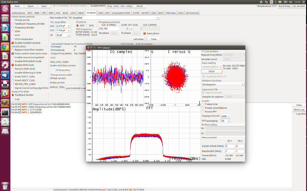
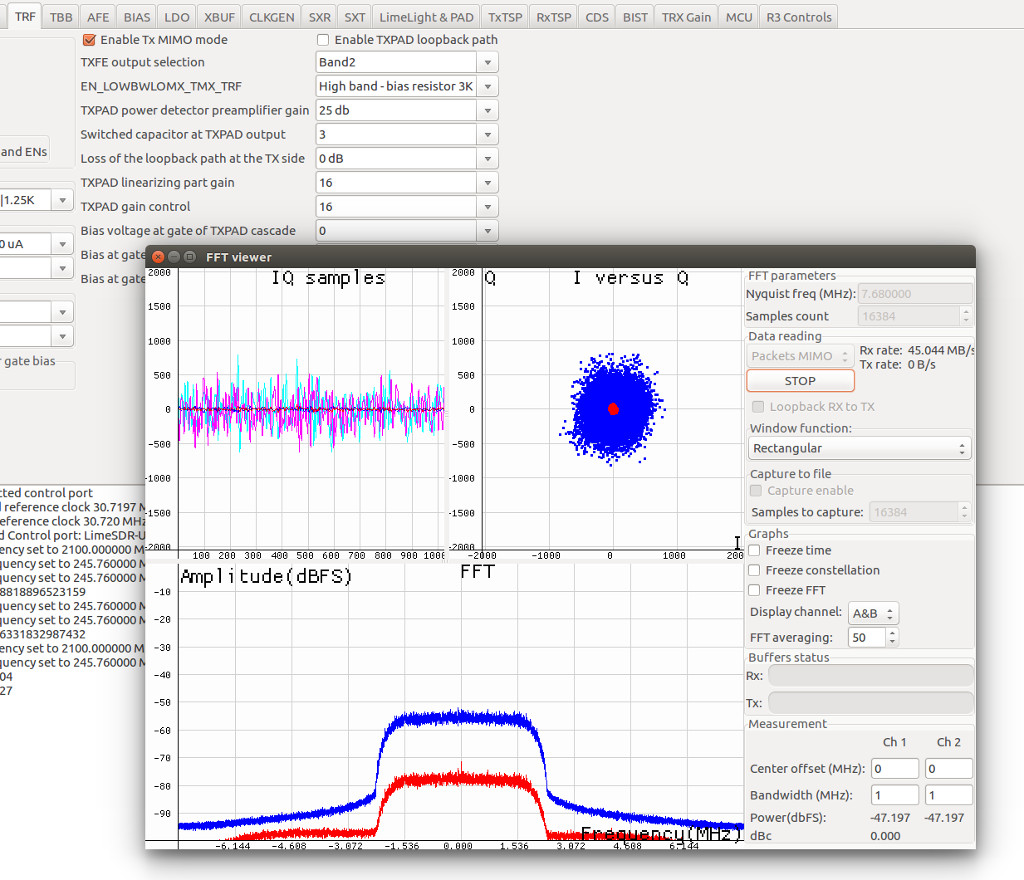
Once at step 3.7 you should have the FFT above, but before we go any further we need to understand what the example has done.
Loading “self_test.ini”
There are over a thousand registers in the LMS7002M, therefore setting them all manually not only would be an inconvenience, it would not make sense. This is where the “.ini” files come in, which contain a list of the LMS7002M register settings and automatically set them, without us having to know or remember them all. If you are interested in what these do there is documentation available here.
Below is a small section of the self_test.ini that we have annotated for an example.
[file_info]
type=lms7002m_minimal_config
version=1
[lms7002_registers_a]
0x0020=0xFFFD < Reset and PWR settings
0x0021=0x0E9F < SPI/I2C control
0x0022=0x07DF < Pad Drive control settings
SXT /SXR
The SXT is the control for the TX PLL and clock generation. It works very similarly to the SXR and so we can discuss these together. For now we shouldn’t need to adjust the parameters other than clicking calculate and tune, but it is best to understand what is happening.
Warning, more background ahead:
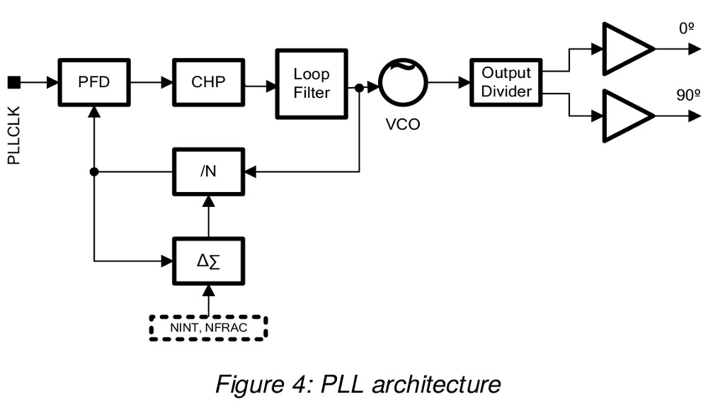
In the last article we discussed the RX PLLs (Phase locked loop) and how they “synthesize a clock”. The reality is the “PLL” part only matches the phase of the clock to another clock source. This “other” clock sources is generated from the reference clock via multipliers and dividers. The PLL’s keep all of these synthesised clocks synchronous so we minimise any phase differences as these will cause phase noise.
If we look at the image of the PLL architecture above we can see the PLL consists of 3 elements:
- Inputs (Nint,Nfract & PLLCLK(ref))
- A feedback loop
- A VCO
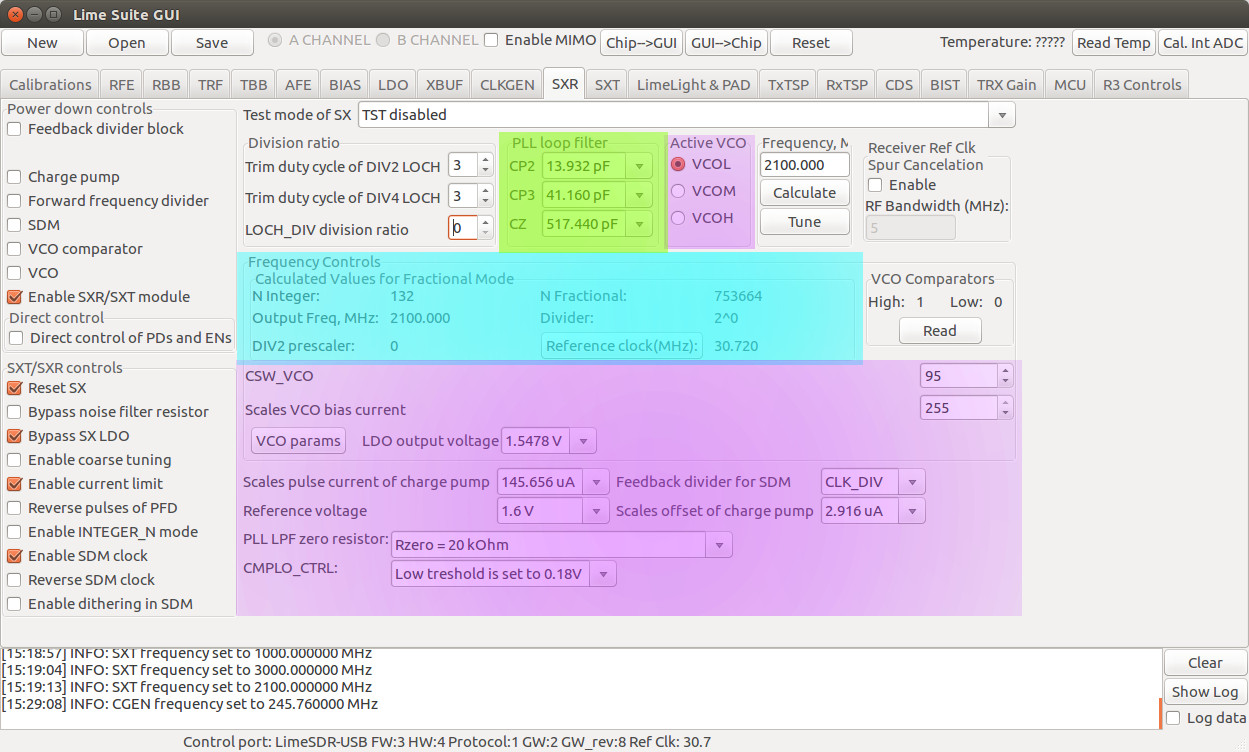
Going back to the self test example, if we are observant when clinking the “Calculate” button a lot of the controls within this tab are adjusted. A good experiment at this time is to try changing the frequencies a few times and see which parts change (remember to change back or reset before continuing)
CLKGEN
The clock generation is very similar to the process described above, but is used to drive the digital side of the LMS7002M, therefore has different parameters that must be optimised. The aim here is to oversample the transmit DACs to improve SNR — higher clock rates are generally better.
Loopback
This is a fairly self-explanatory and it switches over the SKY13323 RF ICs to loopback mode.
Loading the WCDMA waveforms
A part of the FPGA’s role is to provide waveform playback, which as it says on the tin plays a waveform of a known type into the LMS7002M in the correct format.
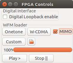
When we load the waveform it’s important to tick MIMO so that the waveform is played from both TX channels. The WCDMA button will not work if the files are not where Lime Suite expects them to be. If you run into this issue, use the “Custom” waveform option to load the WCDMA waveform.
Changing parameters
Finally we can get onto (de)tuning the signal. So that the changes are easy to see we will adjust channel A while leaving channel B alone. Again, if you are following the example along at this point make sure you are back the the “self test” state with both waveforms looking similar. This waveform should have an I/Q plot with a “shotgun” pattern. Currently both channels should be the same, but we can soon adjust that.
Before we get started a point to note is that some tabs adjust both channels (A and B) together, with the SXT asan example of this. We previously looked at the architecture of the LMS7002M to help understand some of these nuances and because we have done this background work we can see the PLL is a shared block, therefore the controls adjust both channels. See, that boring background stuff is starting to pay off!
Since the TX seems OK for the moment, let’s play with some of the RX parameters we discussed in this previous post. If we look closely at the I/Q graph we can notice quite a large pattern (ideally it should fill the plot). If we had a different constellation diagram, such as QAM64, we would be very unhappy with this plot as we’d be looking for discrete dot clusters. It is worth knowing what constellation diagram you are looking for as it will help with the tweaking — or more likely breaking and then finally improving — of your waveforms.
Adjusting the gain
We know the first stage in the LMS7002M is the LNA, so let’s adjust that — it’s currently set at “GMAX”, which is the maximum. Reducing this to GMAX-12 we can see the constellation starts to look a lot more solid. This means we are starting to lose desired information.

So reducing the input is one way of causing this, however can we not just turn down the TX and get the same result? Lets try. Set the RX LNA back to GMAX and adjusting the “TX PAD gain control” to 16 which is part of the TX LNA (in tab TRF).
Almost the same result. There is also a “frontend gain” in the TBB tab, which adjusts the baseband gain. So now let’s try a combination of settings. Set the TXPAD to 12 (TRF tab) and adjust the frontend gain to 60 (TBB tab) to recreate the original gain.
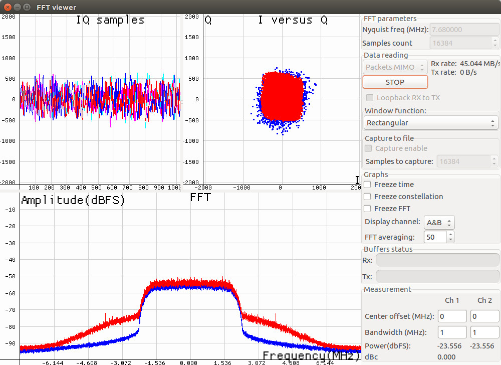
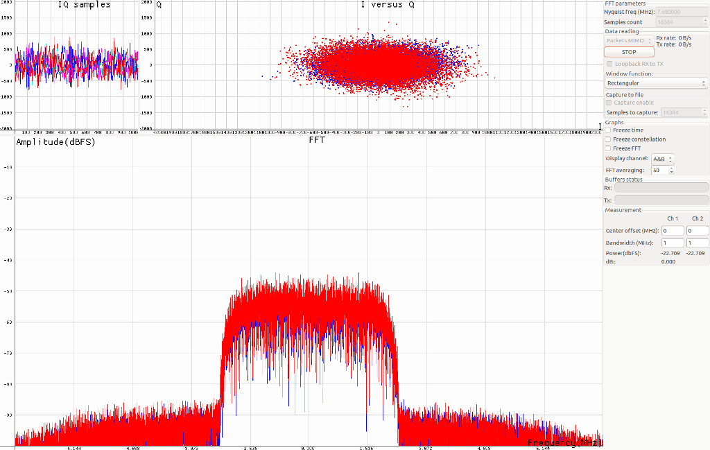
Yikes, we have gain but look at the distortion! Not only have we closed the constellation to a single (but large) point, we are no longer a good neighbour and spreading out into adjacent channels. What’s happened — why have these appeared?
We have just over-driven the filters and you may also notice some severe distortion of the I/Q constellation (it’s been squared off). There are even a few spurious side-bands appearing. These are obviously not good settings, but as an entry into a bad setup competition this could be a winner. As a general rule we should only need to adjust the TXPAD once the other controls are set. Which they are from our “self_test.ini” file, so using gives us a head start. This is also the case for the RX gain controls; we’ve not touched and the TIA and PGA gain controls, however it is probably best to leave these for most cases.
Filters
Dropping back to the “self_test.ini” (load the file and Calculate/Tune TX and CLK again). We know the second stage in both the TX and RX are filters what does adjusting these do?
TBB (TX filter stage controls)
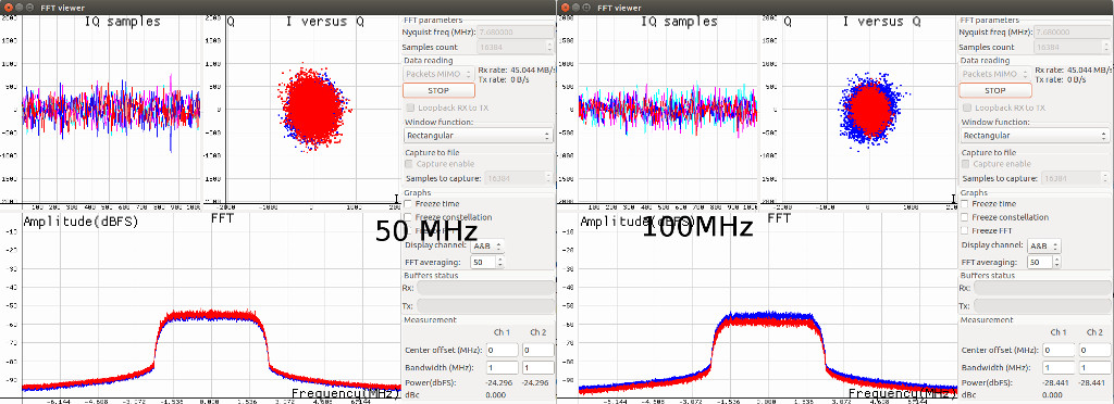
Currently we have a TX filter of 52MHz set, while we can adjust the TX filter values manually we will likely just mess things up (again). Luckily, down at the bottom is another “Tune” button which will automatically calculate the filter coefficients. Typing in 100MHz and clicking Tune you should get a slightly closed I/Q plot, since we are letting more noise though. Note we are using the TXLPFL filter in this example.
We can also bypass the filters by un-ticking LPFLAD_TBB and LPFS5_TBB. This gives the largest constellation yet. One small snag is we’ve stamped all over the adjacent channels as we have no filtering of the higher order harmonics any more. It would be wise not to transmit this signal as it’s likely to cause adjacent channel problems and the authorities are likely to be knocking at your door. Remember to re-apply the filters and set the filters back to 52MHz after this step.
RBB (RX filter stage controls)
This is the control that will be of most interest to those receiving OTA signals, as they will likely need some filtering to improve the reception. Here is a disadvantage of using a clean signal like the WCDMA waveform. For example, we can remove the 10MHz input filter entirely and notice little difference by selecting “LPF_Bypass”.

Manually adjusting the input filters is a little easier to understand as they are presented as RC filters. Re-selecting the LPFL and increasing the capacitor value to 1200, we can see that the waveform is severely distorted because we are dropping higher frequency information in the filter. While we can manually tune these filters it’s still wise to stick to the automatically selected values, just like the TX for most cases. Clicking tune should restore the original settings.
Final words
At this point we’ve touched most of the blocks we’ve previously described. While there are many controls we’ve still not touched or discussed — which include the Bias settings, ADC/DAC blocks and the digital side of the LMS7002M — it’s likely that these settings will be of far less importance to new users, so can wait for another time.
In most cases all we have done is make the signal worse, but understanding what makes something worse will lead to understanding what makes it better too!
In the next article we’ll look at a few applications and possibly optimising rather than breaking them, with the aim of having the confidence to know how to achieve our goals with the LimeSDR.
Karl Woodward