Receiving and transmitting ASK/OOK signals in GNU Radio
Welcome to the seventh instalment of LimeSDR Made Simple. In this post we pick up where we left off in the previous, trying to mimic the simplest of radio devices. In the last instalment we got to a point where we could receive the bit stream, but the number of bits per symbol was incorrect.
In this post we plan on finishing our ASK receiver and providing a transmitter to replay the data!
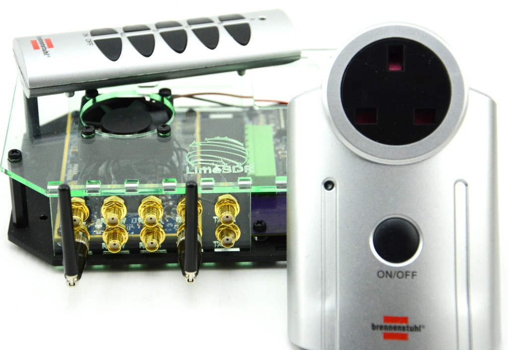
To facilitate this we need to have both a transmitting device (like the keyfob we used last time) and a receiving device. We happened to have a few Brennenstuhl Primera-Line remote controlled extension sockets lying around. Out of curiosity we tried the remote from these and they are ASK and better still, OOK — a simple task of adjusting our flow diagram to match.
Where we left off

The flow graph above is where we left off last time, if you missed this instalment and would like to catch up, the link is here<link>. Before we go too far we should re-cap on what this graph is doing and how some of it works.
- An osmocom source is our LimeSDR
- A “DC blocker” removes the DC component from the received signal. This block is only so the Scope Sink will not have a large DC component displayed.
- The “Multiply const” block provides a fixed digital gain of 10.
- The “RMS” block then averages the signal from sine wave bursts to binary
- The “Add const” block adds a DC offset to move the signal so that it crosses zero, which is required for the “Clock recovery” module
- The “Clock recovery” module and “Binary slicer” then recover the data and record it to a file.
AM demodulation
The RMS block we are using as a AM decoder seems to work, but why?
If we look at the RMS block, it’s quite a simple function: the output is the square root of the average an (Out = sqrt(Avg)). The average is: Avg = (1-Alpha)*Avg + Alpha*abs(in)^2, which in our case since Alpha=1 is: abs(in)^2.

If we take the absolute value of a sine wave we end up with the following waveforms and averaging these waveforms over 10 samples we get:
- Sinewave ≈ 0
- Abs(sine wave)= 0.5
From this it’s clear how the RMS block is magically demodulating the AM signal; when there is a carrier the RMS block output is greater than zero, when there is no carrier the output equals zero.
The clock recovery module
As we discovered in the last instalment, decoding of bits programmatically is much harder than visual decoding OOK waveforms. Due to the bits having a set baud rate we have to sample at the correct time to decode the bit stream. To make this possible we used the clock recovery module, we left off last time just as we had the module proving several bytes per bit. We did leave with the knowledge that these issues we caused by our Omega value being incorrect. The Omega value is the number of samples per bit (which via some math equates to the baud rate).
How do we find the number of samples per bit?
First we need to know the approximate bit length for a single bit. There are a few ways to achieve this and the simplest way is to read a datasheet. In our case we don’t have this information so we must measure it. A program like Universal Radio Hacker (URH) could be used to speed up this process, but there are ways within GNU Radio too.
On some devices the baud rate can vary causing issues. Looking back at the previous eBay keyfob, this was the case and was making things difficult, so we moved on to our new UHF power switch.
With the new Brennenstuhl power switch we had no such issues. By adding a Scope sink after the RMS block and measuring the length of the smallest pulses we can work out the exact Omega value without guess work. In our case the time between the positive and negative edges of a pulse is approximately 0.51ms. Our sample rate is 1MegaSample/Second therefore 1 sample every 1×10⁻⁶ seconds…. Therefore in 0.51ms we get 510 samples our new Omega value.
Before we go ahead and put 510 in the clock recovery module it’s not a good idea to have such a large value in Omega. It would be smarter to down sample before the clock recovery module. Adding a Rational Resampler with a decimation of 10 will reduce our samples per symbol to 51, a much more reasonable value for Omega.
Bit streams are the key (quite literally)
At this point we have a working decoder for our UHF power switch, from this we can decode both the on and off buttons, which give the following bit streams:
Every transmission (including repeats) has a preamble: 11111100000000000000
Off button payload:110100110110110110100110100110110110100110110110100100110100110110100100111111
On button payload: 110100110110110110110110110100100110110110110100100110100110110110100100111111
There are very few differences between the on and off keys. Given the pattern of differences it’s quite likely the bit stream is employing some form or data/inverse data algorithm to provide coding gains and immunity from interference.
Building a transmit flow

It’s all well and good knowing what the data is to turn our Brennunstuhl device on or off, but without a method to transmit this it does us no good. Let’s create a 433MHz OOK transmitter and repeat the sequence we just observed.
The first item in out transmit flow will be our data. Just like when receiving and decoding the data there are many ways to store it. Due to the convenience factor we chose to use the Vector Source over a file storage or message box. Encoding our data in a vector it looks like this: (1,1,0,1…lots_more…,0,0,1). We added 15 leading zero’s as padding so the repeat would have a pause between.
This vector source will continuously playback the bit stream, but at the rate the flow diagram is set to — in our case 1MSample/second — it would be playing 510 times too fast! We could encode a massive vector, so each bit had 510 bits, e.g. “1” turns to 1111…502more…1111. Not an elegant solution. A better way is to use a “Repeat Interpolation” block, which will repeat each bit by the interpolation length (in our case 510 samples), effectively doing the same thing.
Next we can try to set the approximate bit rate by using a “Throttle” block set at 1MSample/second. This block will try to limit the samples, slowing our input to the desired baud rate. At this point we have a square wave output at the correct baud rate — this is a digital signal and does not have a carrier wave so cannot be transmitted.
First we need a carrier and a 433.91MHz sine wave should suffice. The “Signal Source” can create this. Here comes the beauty of OOK signals: by their nature they are on (value 1) or off (value 0), which makes encoding them with a carrier an extremely simple act of multiplication.
Adding a gate is a good idea. Using a “GUI Chooser” set to 0 (default) or 1 allows us to permit or gate the signal via another multiplication block and even provide digital gain if required. All controlled from a button in our flow graph.

The final stage is to add an Osmocom Sink with the correct settings and we have a working radio:
- Device Arguments: “driver=lime,soapy=0”
- Frequency: 433.91e6
- Bandwidth: 5.1e6 < We had to set this as our GNU Radio kept picking an incorrect value and failing to generate a flow.
Before clicking go, be aware that while the 433MHz band is licence exempt there are legal power limits that must be obeyed and turning the RF gain down or using a smaller antenna is advised to stay within these limits. If in doubt start with a low gain setting.
On this topic it is a common misconception more gain is better. This is not always the case e.g. when a device is right next to the transmission source too much gain will just swamp the receiver and make reception worse.
Final words
We hope this instalment of LimeSDR Made Simple demonstrates the power of a LimeSDR and GNU Radio; we have re-created the remote control for our power control switch with just a few simple flowgraphs. This could be true of any OOK device, including your neighbour’s door bell, so please use this power responsibly. While our 433MHz fascination is coming to an end, we may re-visit with FSK or PSK, for the sake of variety we may try something different next time.
Karl Woodward