This is the fifth instalment of LimeSDR Made Simple and in the last we explored the software side of the software-defined radio, using the relatively simple to use dataflow programming environment, Pothos. Quite a break from the previous articles where we went into detail of the input stages of the LimeSDR.
This time we will try to look a little deeper under the hood at some code based examples.
A quick recap
Software-defined radio (SDR) is defined on Wikipedia as:
“a radio communication system where components that have been typically implemented in hardware (e.g. mixers, filters, amplifiers, modulators/demodulators, detectors, etc.) are instead implemented by means of software.”
Now is probably a good time to look back at what we have learned so far:
Part1: Introduction & Part 2: Matching and LMS7002M
In these posts we looked at the RF parts of the software-defined radio, which are implemented in hardware.
Part 3: A practical Example
In this post we started to look at some of the tuning parameters associated with the hardware part of the SDR. This would be the last stage that data would be processed in pure hardware and any additional stages would be within the software domain (In specialist cases the FPGA may be used too).
Part 4: to Pothos and Beyond
This is where things get really fluid. Up until this point we are restricted by hardware blocks that are in the physical world. While seemingly miraculous and capable of tuning from 100kHz to 3.8GHz, the hardware must be implemented in silicon and is therefore limited to what this allows.
This part is where the software came in: we added filters, demodulators and detectors within the FM example all — within the software domain.
A disconnect
Between parts 3 and 4 there was something of a disconnect, as we went from using Lime Suite GUI to Pothos, since the latter is a very high level software environment and as such most of the low level parameters are assumed or abstracted away. How do we know what settings are enabled and is there something in between?
To this extent let’s start to look at something that unearths more of the LMS7002M controls.
Into deeper waters
With the desire to dig a little deeper comes more complexity. However, if you’ve managed to chew though all of the maths of the previous articles and still come back for more, it’s likely this complexity is what you desire. So without delay let’s introduce GNU Octave. Octave is an open source MATLAB-style mathematical language and programming environment. If you have a desire for experimentation in complicated mathematics that would make most mortals cringe in fear then look no further. Octave will become your language of choice and for those of us on the less mathochistic side of the fence, fear not as examples are provided and the language is quite user friendly.

If you plan on working along or wish to use Octave in the future the install is a little more involved than with Pothos or Lime Suite. Install instructions have been included here and please follow these carefully, as there are quite a few steps. We will be working though the ASK demo, which was created for a hackathon and is more of a beta quality than release software.
At the time of writing these demos were working in the windows environment. Linux is untested at present as there were a few issues on our machine, but it should be possible to make it work.
One point if you decide to go ahead with using Linux is to make sure to install all of the packages. These include signal and communications, along with the Lime packages. Additional to the instructions you should install gnuplot via “sudo apt-get install gnuplot” and without this you may get an error. This was certainly the case on a fresh install of Ubuntu.
If you have download the workshop files from the link above a point to note: only the ASK and FSK demos are safe to run without specialised EMI screening or a licence. The other demos are cellular and will require you to have a licence to use the spectrum they transmit upon.
GNU Octave
The whole reason we’ve installed all of these applications is to explore the software side of SDR and Octave should fit this purpose nicely. Before we get started on any SDR specifics an overview of this extremely powerful package is required. MATLAB and therefore Octave, were originally designed to solve mathematical equations. This makes it ideal for prototyping the software part of SDR to synthesise “mixers, filters, amplifiers, modulators/demodulators, detectors, etc.” in software. We need maths and in some cases lots of maths!
Taking the simplest example in software of a gain stage, once the signal is in the digital domain simply multiplication (gain) or division (loss) will achieve our goal. While a very simple concept, implementation can be an issue due to the amount of samples we have producing a very large matrix of complex numbers. Dealing with these matrices in Python or C can be a pain as these would turn into multi-dimensional arrays at this point. C can start to become “fun” to keep track of.
Octave/MATLAB (MATrix LABoratory) is designed with matrices maths in mind and this becomes very simple. To prove this point let’s make a sine wave I and it’s Q component. This code can either be made into a program of manually typed into the command line:
From this small fragment of code we can generate a sine wave of any frequency. Simple, however this is not I/Q data and so we need a little modification. Note the “j” notation for complex numbers:
![]()
plotting these gives us:
![]()

At this point if we wish to ½ this waveform: iqsinehalf = iqsine/2. Thus is the power of a mathematical language.
While doing the mathematics of creating signals ourselves is fun, Octave has an amazing array of tools to assist in the creation/modulation of waveforms. E.g. within the communications package there is a command “fmmod”, which as you may have guessed by the title, will provide FM modulation.
The signal package provides filters and measurement tools like FFT and spectrographs. If you wanted a software package to use with your SDR for waveform research and development you’d be hard pushed to find a more capable program.
If you’re not sold on the power of Octave yet, ponder this question while we work on the ASK demo: where can we get waveform files to play out of the TX?
Amplitude Shift Keying (ASK)
ASK is a common encoding technique in the simplest of radio devices, with an example being a key fob for your garage door. The technique is simple — so simple it can be understood and human readable from a single waveform. The data 1101 0010 is encoded below, with a one being represented by tone and zero by absence of tone.

As can be seen this is a very simple technique. In addition, since this technology is commonly used in licence free bands it makes it the obvious starting point for a transmit example.
Important: do note that while the 866MHz frequency is licence free in the UK, this not universal and the example may need to be changed to match the local regulations. Within Europe there is a maximum transmit power within this band, so just like the other examples remove any high gain antenna and consider using the loopback or a cable if you are unsure.
At this point load ASK.m and depending on your installation you may need to add a line of code to the example:
After the line “pkg load communications” add “pkg load limesdr”.
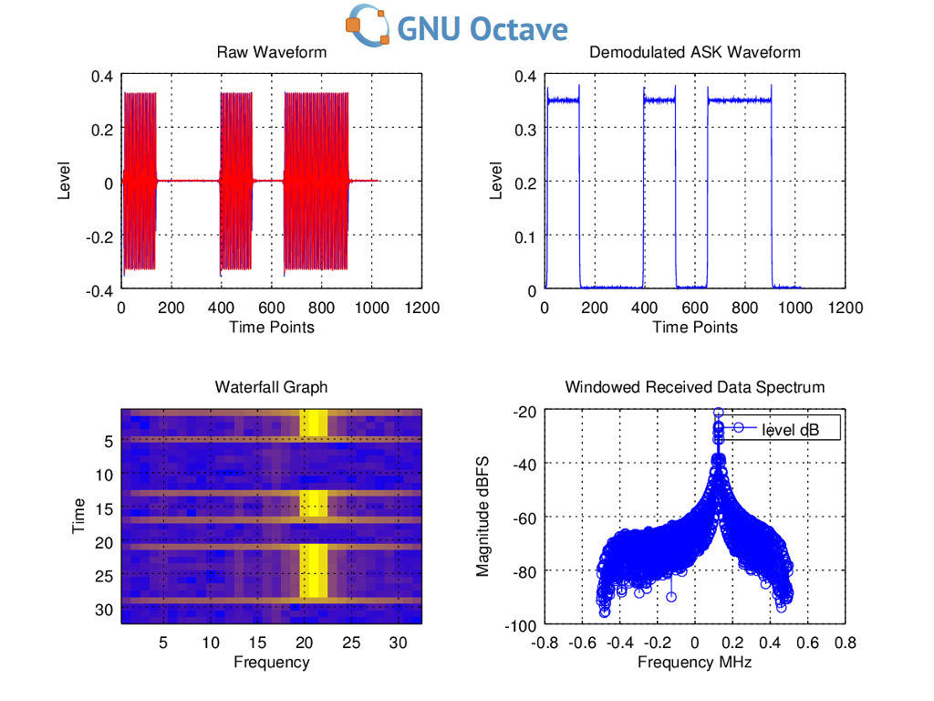
Then when running the example you should get the following waveform out. You can also test this without using your LimeSDR, by setting “useLimeSDR=false;”

Still a black box
I hear you screaming, I’m still non the wiser — what is going on?! Well let’s have a look now at what is going on under the hood. We can see a file in the directory that should be familiar from Part 3 of LimeSDR Made Simple, the “.ini” file. If we look in the .m file we can see this file being called and passed as the “LimeLoadConfig” variable.
So how do we alter the settings? Simple, open the .ini in LimeSuiteGUI and adjust them just as we did the self-test.ini (well not exactly the same, as we broke everything in that instalment!) Changing the TX frequency sample rate and filters should be exactly the same as we did previously, which is why we put ourselves through the background work to start with.
Up until this point the examples have been running in a Windows environment. Octave support is somewhat experimental and issues are to be expected until the kinks are ironed out. This was the case when the demo was run under Linux and we could receive but not transmit.
Note the large amount of variables created after running the example. Looking at these there are some of interest, e.g. iqDataTx and iqDataTxo, with the latter being an oversampled version of the first. Oversampling is a good idea because it reduces the chance of aliasing since it moves them further away from the fundamental, reducing the filtering requirements in the TX path.
Looking at the octave example we can break the code into a few sections:
Variable and waveform creation

Lime start-up controls

Receiving waveforms
![]()
Lime shut-down controls

All the other code is associated with manipulating the data for graphing/readability. The key controls here are the start-up, which includes a transmit method, and the receive which includes how to receive. Note that if you wish to only transmit a single instance of the waveform there is a “LimeTransmitSamples” command that works like the receive command.
Final words
We’ve tested another way of receiving and even transmitting from our LimeSDR. We’ve also introduced a very powerful tool for DSP and the “software” part of SDR. By using this method it helps bridge the void between the hardware and software parts of the radio, as we can see the .ini files being pushed towards the hardware. Next time we will try more transmitting from our LimeSDR, but hopefully without so much coding or maths, although we give no promises.
Karl Woodward